Voltage synthesis (setigen.voltage)
The setigen.voltage module extends setigen to the voltage regime. Instead of
directly synthesizing spectrogram data, we can produce real voltages, pass them
through a software pipeline based on a polyphase filterbank, and record to file
in GUPPI RAW format. setigen.voltage can also reduce those RAW files to
filterbank data products directly with reduce_raw(),
writing either .fil or .h5 output without requiring an external
rawspec installation. As this process models actual hardware used by
Breakthrough Listen for recording raw voltages, this enables lower level
testing and experimentation.
A set of tutorial walkthroughs can be found here.
The basic pipeline structure
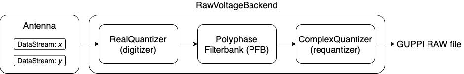
The basic layout of a voltage pipeline written using setigen.voltage
is shown in the image.
First, we have an Antenna, which contains DataStreams for each polarization (1 or 2 total). Noise and signals are added to individual DataStreams, so that polarizations are unique and not necessarily correlated. These are added as functions, which accept an array of times in seconds and return an array of voltages, corresponding to random noise or defined signals. This allows us to obtain voltage samples on demand from each DataStream, and by extension from the Antenna.
The main backend elements are the digitizer, filterbank, and requantizer. The digitizer quantizes input voltages to a desired number of bits, and a desired full width at half maximum (FWHM) in the quantized voltage space. The filterbank implements a software polyphase filterbank, coarsely channelizing input voltages. The requantizer takes the resulting complex voltages, and quantizes each component to either 8 or 4 bits, suitable for saving into GUPPI RAW format.
All of these elements are wrapped into the RawVoltageBackend, which connects
each piece together. The main method
record() automatically
retrieves real voltages as needed and passes them through each backend element,
finally saving out the quantized complex voltages to disk.
A minimal working example of the pipeline is as follows:
from astropy import units as u
import setigen as stg

antenna = stg.voltage.Antenna(sample_rate=3e9*u.Hz,
                              fch1=6000e6*u.Hz,
                              ascending=True,
                              num_pols=1)

antenna.x.add_noise(v_mean=0,
                    v_std=1)

antenna.x.add_constant_signal(f_start=6002.2e6*u.Hz,
                              drift_rate=-2*u.Hz/u.s,
                              level=0.002)

digitizer = stg.voltage.RealQuantizer(target_fwhm=32,
                                      num_bits=8)

filterbank = stg.voltage.PolyphaseFilterbank(num_taps=8,
                                             num_branches=1024)

requantizer = stg.voltage.ComplexQuantizer(target_fwhm=32,
                                           num_bits=8)

rvb = stg.voltage.RawVoltageBackend(antenna,
                                    digitizer=digitizer,
                                    filterbank=filterbank,
                                    requantizer=requantizer,
                                    start_chan=0,
                                    num_chans=64,
                                    block_size=134217728,
                                    blocks_per_file=128,
                                    num_subblocks=32)

rvb.record(output_file_stem='example_1block',
           num_blocks=1,
           length_mode='num_blocks',
           header_dict={'HELLO': 'test_value',
                        'TELESCOP': 'GBT'},
           load_template=True,
           verbose=True)
Note the load_template argument, which fills unspecified keys from
setigen’s built-in default RAW header specification before backend-specific
fields are overwritten.
Reducing RAW data to filterbank products
For the common single-product reduction path, RAW data can be reduced directly in Python:
spec = stg.voltage.RawReductionSpec(fftlength=1024,
                                    integration_factor=4,
                                    pol_mode=stg.voltage.PolarizationMode.TOTAL_POWER,
                                    output_format='fil')

stg.voltage.reduce_raw('example_1block',
                       'example_1block.reduced.fil',
                       spec,
                       overwrite=True)
The same reduction is also available on the command line:
setigen-raw-reduce example_1block example_1block.reduced.fil \
  --fftlength 1024 \
  --integration-factor 4 \
  --pol-mode 1 \
  --format fil \
  --overwrite
For notebook/debug workflows, you can also obtain the reduced data directly as
a Frame object:
frame = stg.voltage.reduce_raw_to_frame('example_1block',
                                        spec)
The native reducer supports a single reduction product per call, optional CuPy
acceleration, and rawspec-style polarization semantics for pol_mode=1,
4, and -4. Multi-polarization output products are written to file
directly and are not wrapped in Frame, which remains a
2D total-power interface.
Direct voltage spectrograms
When the desired product is a dynamic spectrum rather than a persistent RAW
file, to_spectrogram() can run
the same exact voltage path and skip the intermediate RAW serialization step.
The backend still generates voltage samples, applies the digitizer, coarse PFB,
and complex requantizer, and then performs fine channelization and integration
directly in Python.
spec = stg.voltage.VoltageSpectrogramSpec(
    fftlength=1024,
    integration_factor=4,
    pol_mode=stg.voltage.PolarizationMode.TOTAL_POWER,
    coarse_method='auto',
    fine_method='auto',
)

result = rvb.to_spectrogram(spec,
                            num_blocks=1,
                            length_mode='num_blocks',
                            verbose=False)
frame = result.to_frame()
The coarse_method and fine_method options accept 'auto',
'full', and 'selected'. Automatic selection is used only for exact
methods that preserve the current channel response and FFT normalization. For
small coarse-channel or fine-channel selections, 'auto' may compute only
the requested DFT bins; otherwise it falls back to the full FFT path.
For targeted analysis, the direct spectrogram and RAW reduction APIs support frequency-region selection on the final fine-channel axis:
roi = stg.voltage.VoltageSpectrogramSpec(
    fftlength=1024,
    integration_factor=4,
    frequency_range=(6001.0e6, 6001.5e6),
    fine_method='selected',
)

frame = rvb.to_spectrogram(roi,
                           num_blocks=1,
                           length_mode='num_blocks',
                           verbose=False).to_frame()
The frequency range is mutually exclusive with start_chan and
num_chans. Existing RAW generation remains available through
record(); direct spectrogram
generation does not write a RAW file unless users separately call
record.
Using GPU acceleration
The process of synthesizing real voltages at a high sample rate and passing through multiple signal processing steps can be very computationally expensive on a CPU. Accordingly, if you have access to a GPU, it is highly recommended to install CuPy, which performs the equivalent NumPy array operations on the GPU (https://docs.cupy.dev/en/stable/install.html). This is not necessary to run raw voltage generation, but will highly accelerate the pipeline.
Once you have CuPy installed, enable GPU acceleration before constructing
voltage objects. It can also be useful to set CUDA_VISIBLE_DEVICES to
specify which GPUs to use. The following enables GPU usage and specifies to use
the GPU indexed as 0.
In Bash:
export CUDA_VISIBLE_DEVICES=0
In Python:
import os
os.environ['CUDA_VISIBLE_DEVICES'] = '0'

import setigen as stg
stg.voltage.set_backend('cupy')
The legacy SETIGEN_ENABLE_GPU=1 environment variable is still supported for
existing scripts. Use stg.voltage.set_backend('numpy') to force CPU
execution.
Details behind classes
Adding noise and signal sources
If your application uses two polarizations, an Antenna’s data streams are
available via the Antenna.x and Antenna.y attributes. For one
polarization, only the former is available. We can inject noise and signal
sources to these individual data streams. Note that you can still add signal
sources after the RawVoltageBackend is created; real voltages are only
computed at execution time.
Real voltage noise is modeled as ideal Gaussian noise. Note that this actually
stores a function with the DataStream that isn’t evaluated until
get_samples() is actually called:
antenna.x.add_noise(v_mean=0,
                    v_std=1)
For convenience, the Antenna.streams attribute is a list containing
the available data streams for each polarization. So, to add a Gaussian noise
source (with the same statistics) to each antenna, you can do:
for stream in antenna.streams:
    stream.add_noise(v_mean=0,
                     v_std=1)
This will adjust the DataStream.noise_std parameter for each
polarization, which is also accessible using
get_total_noise_std().
We can also add drifting cosine signals to each stream:
stream.add_constant_signal(f_start=6002.2e6,
                           drift_rate=-2*u.Hz/u.s,
                           level=0.002,
                           phase=0)
Here, f_start is the starting frequency, drift_rate is the
change in frequency per time in Hz/s, level is the amplitude of the
cosine signal, and phase is the phase offset in radians.
Custom signal sources
To add custom signal source functions, you can use the add_signal
method:
stream.add_signal(my_signal_func)
Signal source functions are Python functions that accept an array of times, in seconds, and output a corresponding sequence of real voltages. A simple example showing how you might generate Gaussian noise “signal”:
def my_noise_source(ts):
    rng = np.random.default_rng()
    return rng.normal(0, 1, len(ts))

stream.add_signal(my_noise_source)
As custom signals are added, the DataStream.noise_std parameter may no
longer be accurate. In these cases, you may run
update_noise() to estimate the
noise based on a few voltages calculated from all noise and signal sources.
Then, the proper noise standard deviation can be produced via
get_total_noise_std().
You may also check out these example notebooks: 03_custom_signals.ipynb and 04_custom_signals_estimate_noise.ipynb.
Quantizers
The quantization classes are RealQuantizer and ComplexQuantizer. The latter actually uses the former for quantizing real and imaginary components independently. Quantization is run per polarization and antenna.
The quantizers attempt to map the voltage distribution to an ideal quantized
normal distribution with a target FWHM. Voltages that extend past the range of
integers representable by num_bits are clipped. The standard deviation
of the voltage distribution is calculated as they are collected, on a subset
of stats_calc_num_samples samples. By default, this calculation is run
on every pass through the pipeline, but can be limited to periodic calculations
using the stats_calc_period initialization parameter. If this is set to
anything besides a positive integer, the calculation will only be run on the
first call and never again (which saves a lot of computation, but may not be
the most accurate if the voltage distribution changes over time).
Polyphase filterbank
The PolyphaseFilterbank class implements and applies a PFB to quantized input voltages. A good introduction to PFBs is Danny C. Price 2016, “Spectrometers and Polyphase Filterbanks in Radio Astronomy” (http://arxiv.org/abs/1607.03579), as well as the accompanying Jupyter notebook.
The main things to keep in mind when initializing a PolyphaseFilterbank object are:
num_tapscontrols the spectral profile of each individual coarse channel. The larger this is, the closer the spectral response gets to ideal.num_branchescontrols the number of coarse channels. After the real FFT, we obtainnum_branches / 2total coarse channels spanning the Nyquist range.
The PFB frontend uses the original row-loop implementation by default for both
NumPy and CuPy backends. A tap-vectorized frontend is available for local
experiments by setting filterbank.frontend_method = 'vectorized', but it is
not enabled automatically because it can increase temporary memory use and is
not guaranteed to be faster for every backend or block size. This frontend
choice is separate from coarse_method='auto' in direct spectrogram
generation, which controls whether the coarse-channel FFT computes all coarse
DFT bins or only selected output bins.
Voltage backend
The RawVoltageBackend class connects the various components in the pipeline, allowing us to “record” only as much data as we currently need.
Behind the scenes, the backend actually uses a separate instance of each
backend element per antenna and polarization. For example, if the backend is
initialized with a single object instance for each the digitizer, filterbank,
and requantizer, the backend object will make deep copies for each polarization
in each antenna. This is done so that quantization (scaling) calculations are
done independently for separate polarizations and antennas. Alternatively, you
can initialize the backend with 2D lists of shape (num_antennas, num_pols) for
each backend element, if, for example, there are variations in the desired
target_mean and target_fwhm parameters.
Creating multi-antenna RAW files
To simulate interferometric pipelines, it may be useful to synthesize raw
voltage data from multiple antennas. The MultiAntennaArray class supports
exactly this, creating a list of sub-Antennas each with an associated integer
delay (in time samples). In addition to the individual data streams that allow
you to add noise and signals to each Antenna, there are “background” data
streams bg_x and bg_y in MultiAntennaArray, representing
common / correlated noise or RFI that each Antenna can see, subject to the
(relative) delay. If there are no delays, the background data streams will be
perfectly correlated for each antenna.
Here’s an example initialization for a 3 antenna array:
sample_rate = 3e9
delays = np.array([0, 1e-6, 2e-6]) * sample_rate
maa = stg.voltage.MultiAntennaArray(num_antennas=3,
                                    sample_rate=sample_rate,
                                    fch1=6*u.GHz,
                                    ascending=False,
                                    num_pols=2,
                                    delays=delays)
You can access both background data streams using the MultiAntennaArray.bg_streams attribute:
for stream in maa.bg_streams:
    stream.add_noise(v_mean=0,
                     v_std=1)
    stream.add_constant_signal(f_start=5998.9e6,
                               drift_rate=0*u.Hz/u.s,
                               level=0.0025)
Then, instead of passing a single Antenna into a RawVoltageBackend object, you pass in the MultiAntennaArray:
rvb = stg.voltage.RawVoltageBackend(maa,
                                    digitizer=digitizer,
                                    filterbank=filterbank,
                                    requantizer=requantizer,
                                    start_chan=0,
                                    num_chans=64,
                                    block_size=6291456,
                                    blocks_per_file=128,
                                    num_subblocks=32)
The RawVoltageBackend will get samples from each Antenna, accounting for the background data streams intrinsic to the MultiAntennaArray, subject to each Antenna’s delays.
You may also check out this example notebook: 01_multi_antenna_raw_file_gen.ipynb.
Injecting signals at a desired SNR
With noise and multiple signal processing operations, including an FFT, it
can be a bit tricky to choose the correct amplitude of a cosine signal at the
beginning of the pipeline to achieve a desired signal-to-noise ratio (SNR) in
the final finely channelized intensity data products.
setigen.voltage.level_utils has a few helper functions to facilitate
this, depending on the nature of the desired cosine signal.
Since the final SNR depends on the fine channelization FFT length and the time integration factor, as well as parameters inherent to the data production, we need external functions to help calculate an amplitude, or level, for our cosine signal.
First off, assume we are creating a non-drifting cosine signal. If the signal
is at the center of a finely channelized frequency bin,
get_level() gives the appropriate cosine
amplitude to achieve a given SNR if the initial real Gaussian noise has a
variance of 1:
fftlength = 1024
num_blocks = 1
signal_level = stg.voltage.get_level(snr=10,
                                     raw_voltage_backend=rvb,
                                     fftlength=fftlength,
                                     num_blocks=num_blocks,
                                     length_mode='num_blocks')
If the noise in the DataStream doesn’t have a variance of 1, we need to adjust
this signal level by multiplying by
get_total_noise_std().
Note that this method also works for data streams within Antennas that are
part of MultiAntennaArrays, since it will automatically account for the
background noise in the array. Since the noise power is squared during fine
channelization, the signal amplitude should go linearly as a function of the
standard deviation of the noise.
If the signal is non-drifting, in general the spectral response will go as
1/sinc^2(x), where x is the fractional error off of the center
of the spectral bin. To calculate the corresponding amount to adjust
signal level, you can use
get_leakage_factor(). This technically
calculates 1/sinc(x), which is inherently squared naturally along
with the cosine signal amplitude during fine channelization.
To account for drift rates, it gets a bit more complicated; in general, if the
drift rate is larger than a pixel by pixel slope of 1 in the final spectrogram
data products, dividing the initial non-drifting power by that pixel by pixel
slope will result in the new power. In other words, if s is the drift rate
corresponding to a final pixel by pixel slope of 1, then a signal drifting by
2*s will have half the SNR of the non-drifting signal. For a given
RawVoltageBackend and reduced data product parameters fftlength
and int_factor (integration factor), you can calculate s via
get_unit_drift_rate(). However, the situation
is much more complicated for drift rates between 0 and s, so setigen doesn’t
currently automatically calculate the requisite shift in power. Note that if
you’d like to adjust the power for drift rates higher than s, you should
adjust the amplitude (level) of the cosine signal by the square root of the
relevant factor.
An example accounting for multiple effects like these:
f_start = 6003.1e6
leakage_factor = stg.voltage.get_leakage_factor(f_start, rvb, fftlength)
for stream in antenna.streams:
    level = stream.get_total_noise_std() * leakage_factor * signal_level
    stream.add_constant_signal(f_start=f_start,
                               drift_rate=0*u.Hz/u.s,
                               level=level)
You may also check out this example notebook: 05_raw_file_gen_snr.ipynb.
Injecting signals starting from existing RAW files
In addition to recording entirely synthetic voltage data, we can also inject signals onto existing RAW files. This approach is somewhat limited, since the data in existing RAW files have necessarily already been digitized, channelized, and requantized using hardware at the telescope; we cannot add the time series real voltage signals.
Instead, we can use parameters from the RAW data to create synthetic data
streams, and add the corresponding complex RAW voltages together as our
“injection”. Of course, we want to make sure the synthetic data properties
match those of the RAW files, so we have a helper function
get_raw_params that returns a dictionary with relevant properties.
Note that we still need to specify which coarse channel the recorded data
starts from, since this isn’t saved in the header.
start_chan = 0
input_file_stem = 'example_snr'

raw_params = stg.voltage.get_raw_params(input_file_stem=input_file_stem,
                                        start_chan=start_chan)

antenna = stg.voltage.Antenna(sample_rate=sample_rate,
                              **raw_params)
To then create a RawVoltageBackend, we use the class method
from_data(), where input_file_stem is the
filename stem as used by rawspec.
rvb = stg.voltage.RawVoltageBackend.from_data(input_file_stem=input_file_stem,
                                              antenna_source=antenna,
                                              digitizer=digitizer,
                                              filterbank=filterbank,
                                              start_chan=start_chan,
                                              num_subblocks=32)
There are a few things to keep in mind here. Since we don’t have access to the
original noise distribution in real voltage space for the recorded RAW data
(as it was quantized), it may be tough to inject at specific SNR levels. Also,
if we create an Antenna with only cosine-like signals, the distribution of
voltages will look highly non-Gaussian. So, if we attempt to digitize or
requantize this normally, we risk distorting the data and introducing
artifacts. To avoid this, if the Antenna has no injected Gaussian noise source,
we can run record() with parameter
digitize=False. Then, the signals will be channelized and quantized as
if they were embedded in zero-mean Gaussian noise with standard deviation 1.
Now, if there is a noise source, you can leave digitize=True
(the default).
rvb.record(output_file_stem='example_snr_input',
           header_dict={'TELESCOP': 'GBT'},
           digitize=False,
           verbose=True)
In the record() call, if no
num_blocks or obs_length is specified, data will be recorded
matching the total length / size of the input data. You may specify these
parameters to record a smaller amount of data (starting from the beginning of
the input), but of course you can’t produce a longer recording than what is
present in the input.
Behind the scenes, at each iteration, the backend will read in a full data block from disk, and set requantizer statistics (target mean, target standard deviation) for each (antenna, polarization) pair for the real and imaginary quantizer components. Then, the synthetic data passing through the pipeline is requantized to the corresponding standard deviations in each complex component, but instead of centering to the target mean, they are centered to zero mean. This is so that when we add the synthetic data to the existing data, we don’t change the overall voltage means. After these are added together, we finally requantize once more with the same requantizers, to the target mean and standard deviations. This procedure is done to match the existing data statistics and magnitudes as best as possible.
You may also check out this example notebook: 06_starting_from_existing_raw_files.ipynb.