Frame methods

Getting frame data

To just grab the underlying intensity data, you can do

data = frame.get_data(db=False)

As it implies, if you set the db flag to True, it will express the intensities in terms of decibels. This can help visualize data a little better, depending on the application.

Plotting frames

There are a variety of options for plotting frames, meant to produce publication-ready images. The main function is plot().

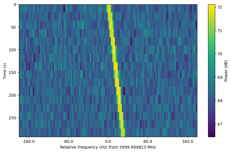
You may choose what style of axes ticks and labels to use with the parameters ftype and ttype. By default, ftype=fmid expresses the frequency axis as the relative offset from the central frequency.

fr.plot()

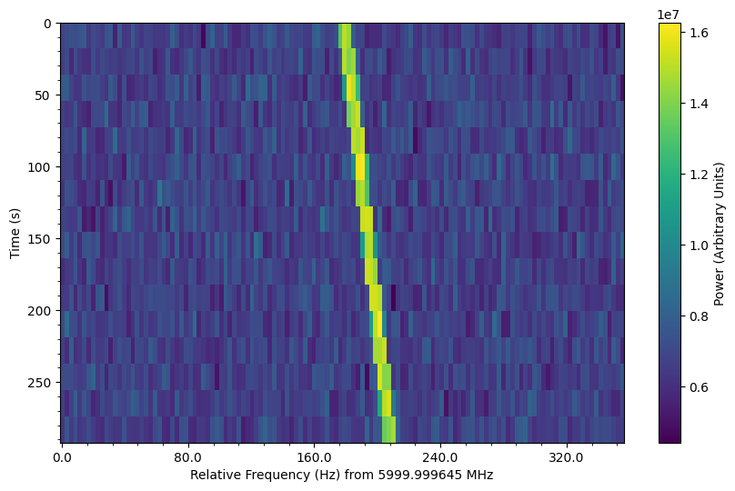
ftype=fmid expresses the frequency axis as the relative offset from the minimum frequency. In addition, we can disable the dB scaling of the colorbar and turn on minor ticks:

fr.plot(ftype="fmin", db=False, minor_ticks=True)

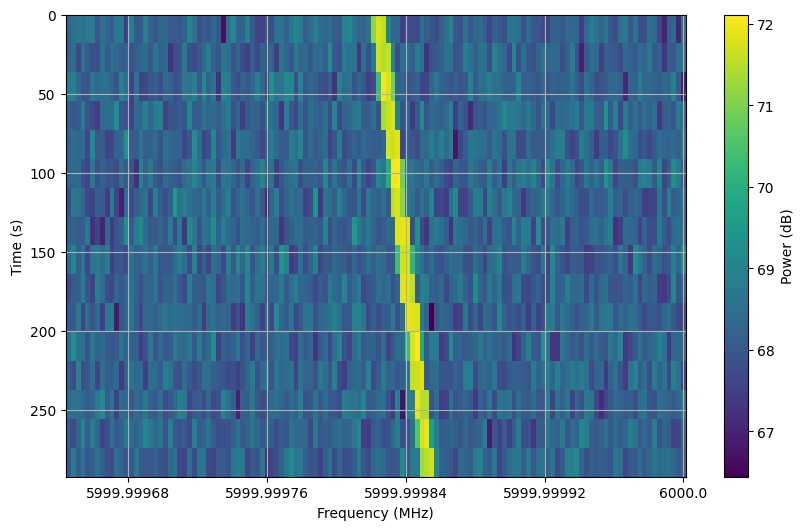
ftype=f expresses the frequency axis as absolute frequencies in MHz. In addition, we can turn on a grid:

fr.plot(ftype="f", grid=True)

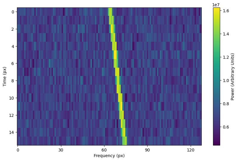
Finally, ftype=px expresses both axes in terms of pixels.

fr.plot(ftype="fmin", db=False)

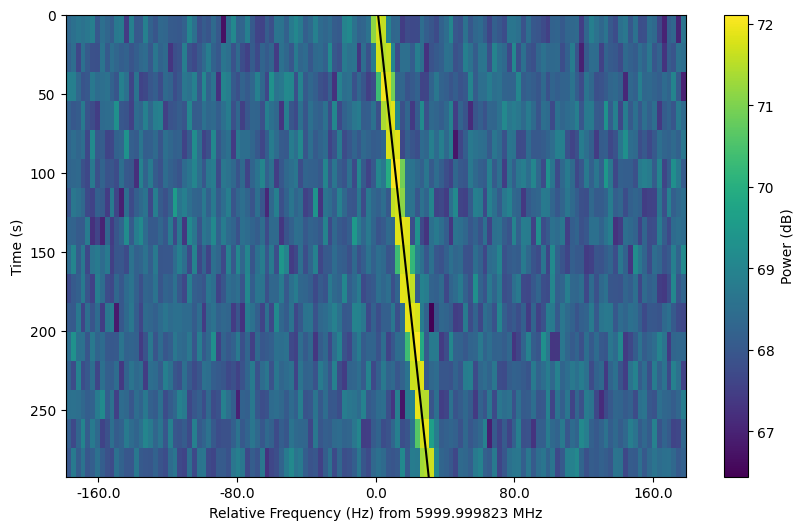
Note that these plots are created using the corresponding units, so that you can actually plot over them in an intuitive way. For example, we can overplot a line following the path of our synthetic signals (frame attribute ts_ext is a time array of length tchans + 1 that includes the end of the frame):

fr.plot(ftype="fmid", db=True)
plt.plot(fr.ts_ext * drift_rate + fr.get_frequency(index=fr.fchans//2) - fr.fmid,
         fr.ts_ext,
         c='k')

The time axis type is ttype="same", by default, which matches the time units to the frequency axis units. You can set the time units to be in seconds relative to the start ("trel") or pixels ("px"). You may also swap the axes by setting swap_axes=True as an optional argument.

The plotting function uses matplotlib.pyplot.imshow behind the scenes, which means you can still control plot parameters before and after these function calls, e.g.

fig = plt.figure(figsize=(10, 6))
frame.plot()
plt.title('My awesome title')
plt.savefig('frame.png')
plt.show()

Frame integration

To time integrate to get a spectrum, or to frequency integrate to get time series intensities, you can use integrate():

spectrum = frame.integrate() # stg.integrate(frame)
time_series = frame.integrate(axis='f') # or axis=1

This function is a wrapper for setigen.frame_utils.integrate(), with the same parameters. The axis parameter can be either ‘t’ or 0 to integrate along the time axis, or ‘f’ or 1 to integrate along the frequency axis. The mode parameter can be either ‘mean’ or ‘sum’ to determine the manner of integration.

Frame slicing

Given frequency boundary indices l and r, we can “slice” a frame by using get_slice(), a wrapper for setigen.frame_utils.get_slice():

s_fr = frame.get_slice(l, r) # stg.get_slice(frame, l, r)

Slicing is analogous to Numpy slicing, e.g. A[l:r], along the frequency axis. This method returns a new frame with only the sliced data. This is useful when chained together with boundary detection methods, or simply to isolate sections of a frame for analysis.

Doppler dedrifting

If you have a frame containing a Doppler drifting signal, you can “dedrift” the frame using dedrift(), specifying a target drift rate (Hz/s):

dd_fr = stg.dedrift(frame, drift_rate=2)

This returns a new frame with only the dedrifted data; this will be smaller in the frequency dimension depending on the drift rate and frame resolution.

Alternatively, if “drift_rate” is contained in the frame’s metadata (frame.metadata), the function will automatically dedrift the frame using that value.

drift_rate = 2
frame.metadata["drift_rate"] = drift_rate
dd_fr = stg.dedrift(frame)