Advanced frame topics
Advanced signal creation
Behind the scenes, add_signal() uses signal parameter
functions to compute intensity for each time, frequency pair in the data. This
is kept quite general to allow for the creation of complex signals. In this
section, we explore some of the flexibility behind add_signal().
Writing custom signal functions
You can go beyond setigen’s pre-written signal functions by
writing your own. For each add_signal() input parameter
(path, t_profile, f_profile, and bp_profile),
you can pass in your own custom functions. Note that these inputs are themselves functions.
It’s important that the functions you pass into each parameter have the correct inputs and outputs. Specifically:
pathFunction that takes in time [array]
tand outputs a frequency [array]t_profileFunction that takes in time [array]
tand outputs an intensity [array]f_profileFunction that takes in frequency [array]
fand a reference central frequency [array]f_center, and outputs an intensity [array]bp_profileFunction that takes in frequency [array]
fand outputs an intensity [array]
For example, here’s the code behind the sine path shape:
def my_sine_path(f_start, drift_rate, period, amplitude):
    def path(t):
        return f_start + amplitude * np.sin(2 * np.pi * t / period) + drift_rate * t
    return path
Alternately, you can use the lambda operator:
def my_sine_path(f_start, drift_rate, period, amplitude):
    return lambda t: return f_start + amplitude * np.sin(2 * np.pi * t / period) + drift_rate * t
These can then be incorporated as:
signal = frame.add_signal(my_sine_path(f_start=frame.get_frequency(200),
                                       drift_rate=2*u.Hz/u.s,
                                       period=100*u.s,
                                       amplitude=100*u.Hz),
                          stg.constant_t_profile(level=1),
                          stg.box_f_profile(width=20*u.Hz),
                          stg.constant_bp_profile(level=1))
To see more examples on how you might write your own parameter functions, check out the source code behind the pre-written functions (setigen.funcs).
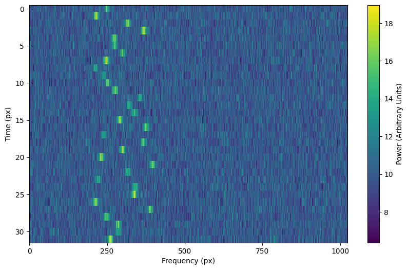
Using arrays as signal parameters
Sometimes it can be difficult to wrap up a desired signal property into a separate function, or perhaps there is external existing code that calculates desired properties. In these cases, we can also use arrays to describe these signals, instead of functions.
from astropy import units as u
import numpy as np
import setigen as stg
import matplotlib.pyplot as plt

frame = stg.Frame(fchans=1024*u.pixel,
                  tchans=32*u.pixel,
                  df=2.7939677238464355*u.Hz,
                  dt=18.253611008*u.s,
                  fch1=6095.214842353016*u.MHz)
frame.add_noise(x_mean=10)

rng = np.random.default_rng()
path_array = rng.uniform(frame.get_frequency(200),
                         frame.get_frequency(400),
                         32)
t_profile_array = rng.uniform(frame.get_intensity(snr=20),
                              frame.get_intensity(snr=40),
                              32)

frame.add_signal(path_array,
                 t_profile_array,
                 stg.gaussian_f_profile(width=40*u.Hz),
                 stg.constant_bp_profile(level=1))

fig = plt.figure(figsize=(10, 6))
frame.plot(ftype="px", db=False)
plt.savefig('frame.png', bbox_inches='tight')
plt.show()
Optimization and accuracy
By default, add_signal() calculates an intensity value for every
time, frequency pairing. Depending on the situation, this might not be the best behavior.
For example, if you are injecting synthetic narrowband signals into a very large frame of data, it can be inefficient and unnecessary to calculate intensity values for every pixel in the frame. In other cases, perhaps calculating intensity values at only every (dt, df) offset would be too inaccurate.
Optimization
To limit the range of signal computation, you can use the bounding_f_range
parameter of add_signal. This takes in a tuple of frequencies
(bounding_min, bounding_max), between which the signal will be computed.
signal = frame.add_signal(stg.constant_path(f_start=frame.get_frequency(200),
                                            drift_rate=2*u.Hz/u.s),
                          stg.constant_t_profile(level=1),
                          stg.box_f_profile(width=20*u.Hz),
                          stg.constant_bp_profile(level=1),
                          bounding_f_range=(frame.get_frequency(100),
                                            frame.get_frequency(700)))
As an example of how this can reduce needless computation, we can time different frame manipulations for a large frame:
import time

times = []
times.append(time.time())

frame = stg.Frame(fchans=2**20,
                  tchans=32,
                  df=2.7939677238464355*u.Hz,
                  dt=18.253611008*u.s,
                  fch1=6095.214842353016*u.MHz)
times.append(time.time())

frame.add_noise(x_mean=10)
times.append(time.time())

# Normal add_signal
frame.add_signal(stg.constant_path(f_start=frame.get_frequency(200),
                                   drift_rate=2*u.Hz/u.s),
                 stg.constant_t_profile(level=frame.get_intensity(snr=30)),
                 stg.gaussian_f_profile(width=40*u.Hz),
                 stg.constant_bp_profile(level=1))
times.append(time.time())

# Limiting computation with bounding_f_range
frame.add_signal(stg.constant_path(f_start=frame.get_frequency(200),
                                   drift_rate=2*u.Hz/u.s),
                 stg.constant_t_profile(level=frame.get_intensity(snr=30)),
                 stg.gaussian_f_profile(width=40*u.Hz),
                 stg.constant_bp_profile(level=1),
                 bounding_f_range=(frame.get_frequency(100),
                                   frame.get_frequency(700)))
times.append(time.time())

x = np.array(times)
print(x[1:] - x[:-1])

>>> [1.14681625 1.4038794  1.6308465  0.02862048]
Depending on the type of signal, you should be cautious when defining a bounding
frequency range. For signals with constant drift rate and small spectral width,
it isn’t too hard to define a range. For example, add_constant_signal()
uses bounding ranges automatically to optimize signal creation.
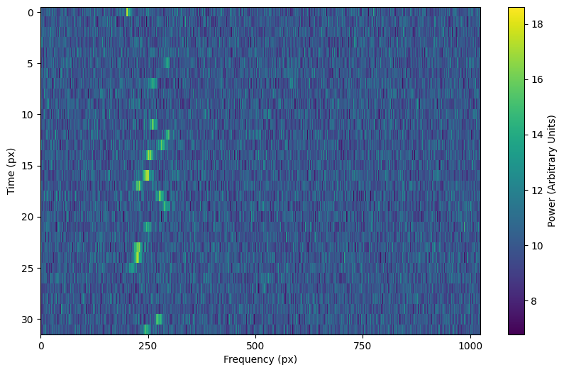
However, for signals with large or stochastic frequency variation, or with long spectral tails, it can be difficult to define a bounding range without cutting off parts of these signals.
To illustrate this, using the above example that takes arrays as signal parameters, setting too small of a bounding frequency range can look like:
frame = stg.Frame(fchans=1024*u.pixel,
                  tchans=32*u.pixel,
                  df=2.7939677238464355*u.Hz,
                  dt=18.253611008*u.s,
                  fch1=6095.214842353016*u.MHz)
frame.add_noise(x_mean=10)

rng = np.random.default_rng()
path_array = rng.uniform(frame.get_frequency(200),
                         frame.get_frequency(400),
                         32)
t_profile_array = rng.uniform(frame.get_intensity(snr=20),
                              frame.get_intensity(snr=40),
                              32)

frame.add_signal(path_array,
                 t_profile_array,
                 stg.gaussian_f_profile(width=40*u.Hz),
                 stg.constant_bp_profile(level=1),
                 bounding_f_range=(frame.get_frequency(200),
                                   frame.get_frequency(300)))
Accuracy
To improve accuracy a bit, we can integrate signal computations over subsamples in
time and frequency. The function add_signal() has three boolean parameters:
integrate_path, integrate_t_profile, and integrate_f_profile,
which control whether various integrations are turned on (by default, they are False).
The former two depend on the t_subsamples parameter, which is the number
of bins per time sample (e.g. per dt) over which to integrate; likewise, integrate_f_profile
depends on the f_subsamples parameter.
integrate_path controls integration of the signal’s center frequency with
respect to time, path. If your path varies on timescales shorter than
the time resolution dt, then it could make sense to integrate to get more
appropriate frequency positions.
integrate_t_profile controls integration of the intensity variation with respect to
time, t_profile. If your t_profile varies on timescales shorter than the
time resolution dt, then it could make sense to integrate to get more
appropriate intensities.
integrate_f_profile controls integration of the intensity variation with respect to
frequency, f_profile. If your f_profile varies on spectral scales
shorter than the frequency resolution df, then it could make sense to integrate
to get more appropriate intensities.
Note that since integration requires make multiple calculations per pixel, it can increase signal computation time significantly. Be sure to evaluate whether it’s actually necessary to integrate, or whether the default add_signal computation is sufficient for your use cases.
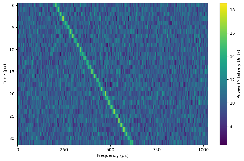
Here is an example of integration in action:
frame = stg.Frame(fchans=1024*u.pixel,
                  tchans=32*u.pixel,
                  df=2.7939677238464355*u.Hz,
                  dt=18.253611008*u.s,
                  fch1=6095.214842353016*u.MHz)
frame.add_noise(x_mean=10)

frame.add_signal(stg.constant_path(f_start=frame.get_frequency(200),
                                   drift_rate=2*u.Hz/u.s),
                 stg.constant_t_profile(level=frame.get_intensity(snr=30)),
                 stg.gaussian_f_profile(width=40*u.Hz),
                 stg.constant_bp_profile(level=1),
                 integrate_path=True,
                 integrate_t_profile=True,
                 integrate_f_profile=True,
                 t_subsamples=10,
                 f_subsamples=10)
Creating custom observational noise distributions
If you are interested in simulating observations of different resolutions and
frequency bands, the underlying noise statistics may certainly differ from the
included C-band distributions used by add_noise_from_obs(). In these cases,
it may be best to generate your own parameter distribution arrays from your
own observations, and feed those into add_noise_from_obs() yourself.
It is worth mentioning that while you can just inject signals into
observational frames directly, real observations may contain real signals as well.
By estimating noise parameter distributions from observations, you can generate
synthetic chi-squared or Gaussian noise with similar noise statistics as real observations,
thereby resembling real data while excluding real signals.
To do this, we can use get_parameter_distributions():
import setigen as stg
waterfall_fn = 'path/to/data.fil'
# Number of frequency channels per frame
fchans = 1024
# Number of time samples per frame; optional
tchans = 32
x_mean_array, x_std_array, x_min_array = stg.get_parameter_distributions(waterfall_fn,
                                                                         fchans,
                                                                         tchans=tchans,
                                                                         f_shift=None)
This will iterate over an entire filterbank file, estimating the noise statistics and returning them as numpy arrays.
Creating an injected synthetic signal dataset using observations
We can create a dataset based on observations using the split_utils
module. We can use split_waterfall_generator() to create
a Python generator that returns blimpy Waterfall objects, from which we can create
setigen Frames. The function get_parameter_distributions()
actually uses this behind the scenes to iterate through observational data.
import setigen as stg
waterfall_fn = 'path/to/data.fil'
fchans = 1024
tchans = 32
waterfall_itr = stg.split_waterfall_generator(waterfall_fn,
                                              fchans,
                                              tchans=tchans,
                                              f_shift=None)
waterfall = next(waterfall_itr)
frame = stg.Frame(waterfall)
Here, f_shift is the number of indices in the frequency direction to shift
before making another slice or split of size fchans. If f_shift=None,
it defaults to shifting over by fchans, so that there is no overlap.
To construct a full dataset, we can then use the generator to iterate over slices of data and save out frames. As a simple example:
for i, waterfall in enumerate(waterfall_itr):
    frame = stg.Frame(waterfall=waterfall)

    rng = np.random.default_rng()
    start_index = rng.integers(0, fchans)
    stop_index = rng.integers(0, fchans)
    drift_rate = frame.get_drift_rate(start_index, stop_index)

    signal = frame.add_constant_signal(f_start=frame.get_frequency(start_index),
                                       drift_rate=drift_rate,
                                       level=frame.get_intensity(snr=10),
                                       width=40,
                                       f_profile_type='gaussian')
    signal_props = {
        'start_index': start_index,
        'stop_index': stop_index,
        'snr': 10,
    }
    frame.add_metadata(signal_props)
    frame.save_pickle('save/path/frame{:06d}.pickle'.format(i))
Depending on the application, it can also pay to save metadata out to a CSV file that tracks filenames / indices with corresponding properties.