Getting started
The heart of setigen is the Frame object. For signal injection and manipulation,
we call each snippet of time-frequency data a “frame.” There are two main ways
to initialize frames, starting from either resolution/size parameters or existing
observational data.
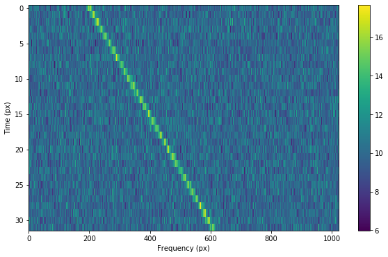
Here’s a minimal working example for a purely synthetic frame, injecting a constant
intensity signal into a background of chi-squared noise. Parameters in setigen are
specified either in terms of SI units (Hz, s) or astropy.units, as in the example:
from astropy import units as u
import setigen as stg
import matplotlib.pyplot as plt

frame = stg.Frame(fchans=1024*u.pixel,
                  tchans=32*u.pixel,
                  df=2.7939677238464355*u.Hz,
                  dt=18.253611008*u.s,
                  fch1=6095.214842353016*u.MHz)
noise = frame.add_noise(x_mean=10, noise_type='chi2')
signal = frame.add_signal(stg.constant_path(f_start=frame.get_frequency(index=200),
                                            drift_rate=2*u.Hz/u.s),
                          stg.constant_t_profile(level=frame.get_intensity(snr=30)),
                          stg.gaussian_f_profile(width=40*u.Hz),
                          stg.constant_bp_profile(level=1))

fig = plt.figure(figsize=(10, 6))
frame.render()
plt.savefig('frame.png', bbox_inches='tight')
plt.show()
This simple signal can also be generated using the method frame.add_constant_signal,
which is optimized for created signals of constant intensity and drift rate in large frames:
frame.add_constant_signal(f_start=frame.get_frequency(200),
                          drift_rate=2*u.Hz/u.s,
                          level=frame.get_intensity(snr=30),
                          width=40*u.Hz,
                          f_profile_type='gaussian')
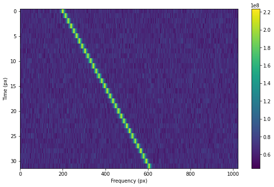
Similarly, here’s a minimal working example for injecting a signal into a frame of observational data (from a blimpy Waterfall object). Note that in this example, the observational data also has dimensions 32x1024 to make it easy to visualize here.
from astropy import units as u
import setigen as stg
import blimpy as bl
import matplotlib.pyplot as plt

data_path = 'path/to/data.fil'
waterfall = bl.Waterfall(data_path)
frame = stg.Frame(waterfall=waterfall)
frame.add_signal(stg.constant_path(f_start=frame.get_frequency(200),
                                   drift_rate=2*u.Hz/u.s),
                 stg.constant_t_profile(level=frame.get_intensity(snr=30)),
                 stg.gaussian_f_profile(width=40*u.Hz),
                 stg.constant_bp_profile(level=1))

fig = plt.figure(figsize=(10, 6))
frame.render()
plt.show()
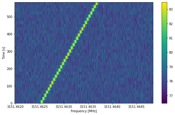
We can also view this using blimpy’s plotting style:
fig = plt.figure(figsize=(10, 6))
frame.bl_render()
plt.show()
Usually, filterbank data is saved with frequencies in descending order, with the first
frequency bin centered at fch1. setigen works with data in increasing frequency
order, and will reverse the data order when appropriate if the frame is initialized with such
an observation. However, if you are working with data or would like to synthesize
data for which fch1 should be the minimum frequency, set ascending=True when
initializing the Frame object. Note that if you initialize Frame using a filterbank file with
frequencies in increasing order, you do not need to set ascending manually.
frame = stg.Frame(fchans=1024*u.pixel,
                  tchans=32*u.pixel,
                  df=2.7939677238464355*u.Hz,
                  dt=18.253611008*u.s,
                  fch1=6095.214842353016*u.MHz,
                  ascending=True)
Assuming you have access to a data array, with corresponding resolution information, you can
can also initialize a frame as follows. Just make sure that your data is already arranged in the desired frequency order; setting the ascending parameter will only affect the frequency
values that are mapped to the provided data array.
my_data = # your 2D array
frame = stg.Frame.from_data(df=2.7939677238464355*u.Hz,
                            dt=18.253611008*u.s,
                            fch1=6095.214842353016*u.MHz,
                            ascending=True,
                            data=my_data)

frame.render()