Basic usage
Adding a basic signal
The main method that generates signals is add_signal().
This allows us to pass in an functions or arrays that describe
the shape of the signal over time, over frequency within individual time samples,
and over a bandpass of frequencies. setigen comes prepackaged with common
functions (setigen.funcs), but you can write your own!
The most basic signal that you can generate is a constant intensity, constant
drift-rate signal. Note that as in the Getting started example, you can also use
frame.add_constant_signal, which is simpler and more efficient for
signal injection into large data frames.
from astropy import units as u
import numpy as np
import setigen as stg
# Define time and frequency arrays, essentially labels for the 2D data array
fchans = 1024
tchans = 16
df = 2.7939677238464355*u.Hz
dt = 18.253611008*u.s
fch1 = 6095.214842353016*u.MHz
# Generate the signal
frame = stg.Frame(fchans=fchans,
tchans=tchans,
df=df,
dt=dt,
fch1=fch1)
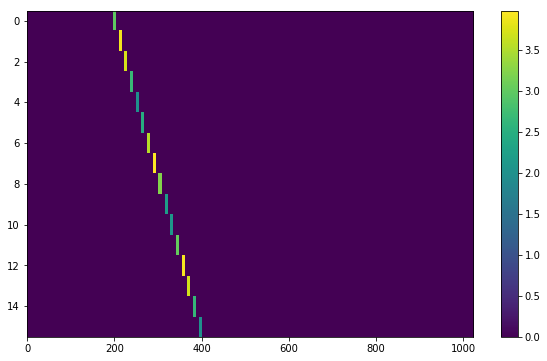
signal = frame.add_signal(stg.constant_path(f_start=frame.get_frequency(200),
drift_rate=2*u.Hz/u.s),
stg.constant_t_profile(level=1),
stg.box_f_profile(width=20*u.Hz),
stg.constant_bp_profile(level=1))
setigen.Frame.add_signal() returns a 2D numpy array containing only the synthetic signal. To
visualize the resulting frame, we can use matplotlib.pyplot.imshow():
import matplotlib.pyplot as plt
fig = plt.figure(figsize=(10, 6))
plt.imshow(frame.get_data(), aspect='auto')
plt.colorbar()
fig.savefig("basic_signal.png", bbox_inches='tight')
In setigen, we use astropy.units to exactly specify where signals
should be in time-frequency space. Astropy automatically handles unit conversions
(MHz -> Hz, etc.), which is a nice convenience. Nevertheless, you can also use normal
SI units (Hz, s) without additional modifiers, in which case the above code would become:
from astropy import units as u
import numpy as np

import setigen as stg

# Define time and frequency arrays, essentially labels for the 2D data array
fchans = 1024
tchans = 16
df = 2.7939677238464355
dt = 18.253611008
fch1 = 6095.214842353016 * 10**6

# Generate the signal
frame = stg.Frame(fchans=fchans,
                  tchans=tchans,
                  df=df,
                  dt=dt,
                  fch1=fch1)
signal = frame.add_signal(stg.constant_path(f_start=frame.get_frequency(200),
                                            drift_rate=2),
                          stg.constant_t_profile(level=1),
                          stg.box_f_profile(width=20),
                          stg.constant_bp_profile(level=1))
So, it isn’t quite necessary to use astropy.units, but it’s an option
to avoid manual unit conversion and calculation.
Using prepackaged signal functions
With setigen’s pre-written signal functions, you can generate a variety
of signals right off the bat. The main signal parameters that customize the
synthetic signal are path, t_profile, f_profile, and
bp_profile.
path describes the path of the signal in time-frequency space. The
path function takes in a time and outputs ‘central’ frequency
corresponding to that time.
t_profile (time profile) describes the intensity of the signal over
time. The t_profile function takes in a time and outputs an intensity.
f_profile (frequency profile) describes the intensity of the signal
within a time sample as a function of relative frequency. The f_profile
function takes in a frequency and a central frequency and computes an intensity.
This function is used to control the spectral shape of the signal (with respect
to a central frequency), which may be a square wave, a Gaussian, or any custom
shape!
bp_profile describes the intensity of the signal over the bandpass of
frequencies. Whereas f_profile computes intensity with respect to a
relative frequency, bp_profile computes intensity with respect to the
absolute frequency value. The bp_profile function takes in a frequency
and outputs an intensity as well.
All these functions combine to form the final synthetic signal, which means you can create a host of signals by switching up these parameters!
Here are just a few examples of pre-written signal functions. To see all of the included functions, check out setigen.funcs. To avoid needless repetition, each example script will assume the same basic setup:
from astropy import units as u
import numpy as np

import setigen as stg

# Define time and frequency arrays, essentially labels for the 2D data array
fchans = 1024
tchans = 16
df = 2.7939677238464355*u.Hz
dt = 18.253611008*u.s
fch1 = 6095.214842353016*u.MHz

# Generate the signal
frame = stg.Frame(fchans=fchans,
                  tchans=tchans,
                  df=df,
                  dt=dt,
                  fch1=fch1)
paths - trajectories in time-frequency space
Constant path
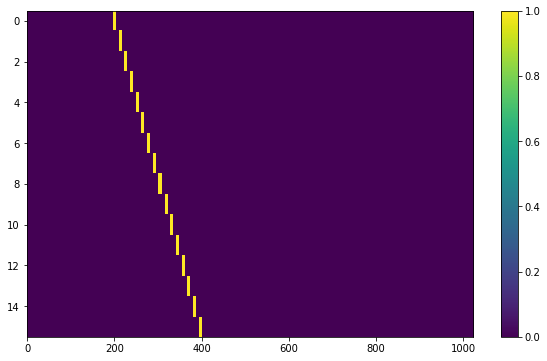
A constant path is a linear Doppler-drifted signal. To generate this path, use
constant_path() and specify the starting frequency of
the signal and the drift rate (in units of frequency over time, consistent with
the units of your time and frequency arrays):
signal = frame.add_signal(stg.constant_path(f_start=frame.get_frequency(200),
                                            drift_rate=2*u.Hz/u.s),
                          stg.constant_t_profile(level=1),
                          stg.box_f_profile(width=20*u.Hz),
                          stg.constant_bp_profile(level=1))
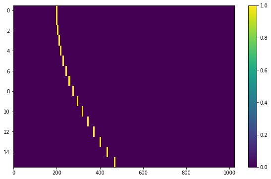
Sine path
This path is a sine wave, controlled by a starting frequency, drift rate, period,
and amplitude, using sine_path().
signal = frame.add_signal(stg.sine_path(f_start=frame.get_frequency(200),
                                        drift_rate=2*u.Hz/u.s,
                                        period=100*u.s,
                                        amplitude=100*u.Hz),
                          stg.constant_t_profile(level=1),
                          stg.box_f_profile(width=20*u.Hz),
                          stg.constant_bp_profile(level=1))

Squared path
This path is a very simple quadratic with respect to time, using
squared_path().
signal = frame.add_signal(stg.squared_path(f_start=frame.get_frequency(200),
                                           drift_rate=0.01*u.Hz/u.s),
                          stg.constant_t_profile(level=1),
                          stg.box_f_profile(width=20*u.Hz),
                          stg.constant_bp_profile(level=1))
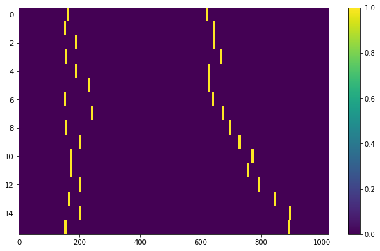
RFI-like path
This path randomly varies in frequency, as in some RFI signals, using
simple_rfi_path(). The following example shows two
such signals, with rfi_type set to ‘stationary’ and ‘random_walk’. You
can define drift_rate to set these signals in relation to a straight
line path.
frame.add_signal(stg.simple_rfi_path(f_start=frame.fs[200],
                                     drift_rate=0*u.Hz/u.s,
                                     spread=300*u.Hz,
                                     spread_type='uniform',
                                     rfi_type='stationary'),
                 stg.constant_t_profile(level=1),
                 stg.box_f_profile(width=20*u.Hz),
                 stg.constant_bp_profile(level=1))

frame.add_signal(stg.simple_rfi_path(f_start=frame.fs[600],
                                     drift_rate=0*u.Hz/u.s,
                                     spread=300*u.Hz,
                                     spread_type='uniform',
                                     rfi_type='random_walk'),
                 stg.constant_t_profile(level=1),
                 stg.box_f_profile(width=20*u.Hz),
                 stg.constant_bp_profile(level=1))
t_profiles - intensity variation with time
Constant intensity
To generate a signal with the same intensity over time, use
constant_t_profile(), specifying only the
intensity level:
signal = frame.add_signal(stg.constant_path(f_start=frame.get_frequency(200),
                                        drift_rate=2*u.Hz/u.s),
                      stg.constant_t_profile(level=1),
                      stg.box_f_profile(width=20*u.Hz),
                      stg.constant_bp_profile(level=1))
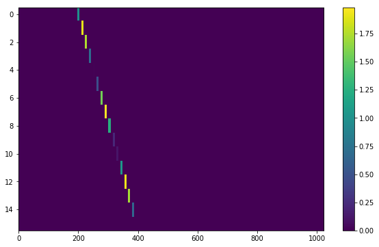
Sine intensity
To generate a signal with sinusoidal intensity over time, use
sine_t_profile(), specifying the period,
amplitude, and average intensity level. The intensity level is essentially an
offset added to a sine function, so it should be equal or greater than the
amplitude so that the signal doesn’t have any negative values.
Here’s an example with equal level and amplitude:
signal = frame.add_signal(stg.constant_path(f_start=frame.get_frequency(200),
                                            drift_rate=2*u.Hz/u.s),
                          stg.sine_t_profile(period=100*u.s,
                                             amplitude=1,
                                             level=1),
                          stg.box_f_profile(width=20*u.Hz),
                          stg.constant_bp_profile(level=1))
And here’s an example with the level a bit higher than the amplitude:
signal = frame.add_signal(stg.constant_path(f_start=frame.get_frequency(200),
                                            drift_rate=2*u.Hz/u.s),
                          stg.sine_t_profile(period=100*u.s,
                                             amplitude=1,
                                             level=3),
                          stg.box_f_profile(width=20*u.Hz),
                          stg.constant_bp_profile(level=1))
f_profiles - intensity variation with time
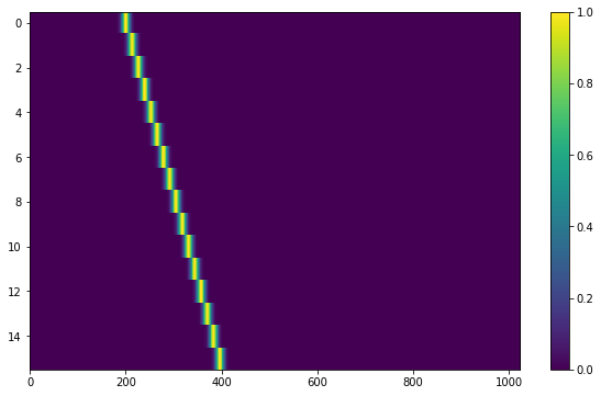
Box / square intensity profile
To generate a signal with the same intensity over frequency, use
box_f_profile(), specifying the width of the
signal:
signal = frame.add_signal(stg.constant_path(f_start=frame.get_frequency(200),
                                            drift_rate=2*u.Hz/u.s),
                          stg.constant_t_profile(level=1),
                          stg.box_f_profile(width=40*u.Hz),
                          stg.constant_bp_profile(level=1))

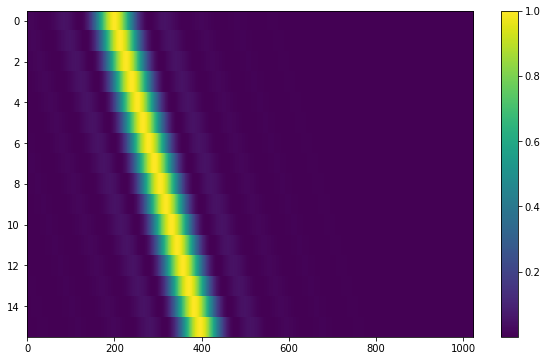
Gaussian intensity profile
To generate a signal with a Gaussian intensity profile in the frequency
direction, use gaussian_f_profile(), specifying
the width of the signal:
signal = frame.add_signal(stg.constant_path(f_start=frame.get_frequency(200),
                                            drift_rate=2*u.Hz/u.s),
                          stg.constant_t_profile(level=1),
                          stg.gaussian_f_profile(width=40*u.Hz),
                          stg.constant_bp_profile(level=1))
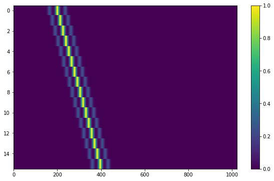
Sinc squared intensity profile
To generate a signal with a sinc squared intensity profile in the frequency direction, use
sinc2_f_profile(), specifying the width of the
signal:
signal = frame.add_signal(stg.constant_path(f_start=frame.get_frequency(200),
                                            drift_rate=2*u.Hz/u.s),
                          stg.constant_t_profile(level=1),
                          stg.sinc2_f_profile(width=40*u.Hz),
                          stg.constant_bp_profile(level=1))

By default, the function has the parameter trunc=True to truncate the sinc squared function at the first zero-crossing. With trunc=False and using a larger width to show the effect:
signal = frame.add_signal(stg.constant_path(f_start=frame.get_frequency(200),
                                            drift_rate=2*u.Hz/u.s),
                          stg.constant_t_profile(level=1),
                          stg.sinc2_f_profile(width=200*u.Hz, trunc=False),
                          stg.constant_bp_profile(level=1))
Multiple Gaussian intensity profile
The profile multiple_gaussian_f_profile(),
generates a symmetric signal with three Gaussians; one main signal and two
smaller signals on either side. This is mostly a demonstration that f_profile functions can be composite, and you can create custom functions like this (advanced.rst).
signal = frame.add_signal(stg.constant_path(f_start=frame.get_frequency(200),
                                            drift_rate=2*u.Hz/u.s),
                          stg.constant_t_profile(level=1),
                          stg.multiple_gaussian_f_profile(width=40*u.Hz),
                          stg.constant_bp_profile(level=1))
Adding synthetic noise
The background noise in high resolution BL data inherently follows a chi-squared
distribution. Depending on the data’s spectral and temporal resolutions, with enough
integration blocks, the noise approaches a Gaussian distribution. setigen
supports both distributions for noise generation, but uses chi-squared by default.
Every time synthetic noise is added to an image, setigen will
estimate the noise properties of the frame, and you can get these via
get_total_stats() and get_noise_stats().
Important note: over a range of many frequency channels, real radio data has complex systematic structure, such as coarse channels and bandpass shapes. Adding synthetic noise according to a pure statistical distribution as the background for your frames is therefore most appropriate when your frame size is somewhat limited in frequency, in which case you can mostly ignore these systematic artifacts. As usual, whether this is something you should care about just depends on your use cases.
Adding pure chi-squared noise
A minimal working example for adding noise is:
import matplotlib.pyplot as plt
import numpy as np
from astropy import units as u
import setigen as stg
# Define time and frequency arrays, essentially labels for the 2D data array
fchans = 1024
tchans = 16
df = 2.7939677238464355*u.Hz
dt = 18.253611008*u.s
fch1 = 6095.214842353016*u.MHz
# Generate the signal
frame = stg.Frame(fchans=fchans,
tchans=tchans,
df=df,
dt=dt,
fch1=fch1)
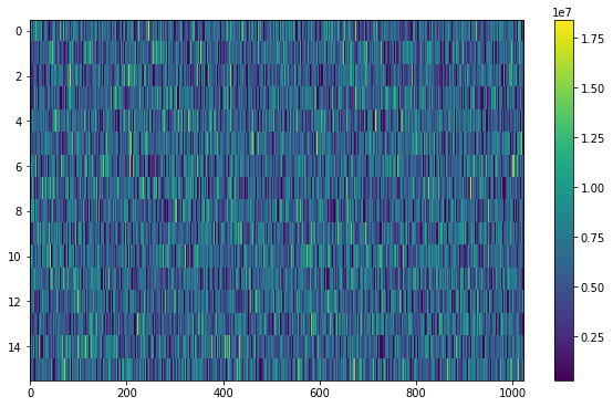
noise = frame.add_noise(x_mean=10)
fig = plt.figure(figsize=(10, 6))
plt.imshow(frame.get_data(), aspect='auto')
plt.colorbar()
plt.show()
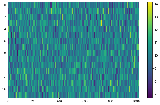
This adds chi-squared noise scaled to a mean of 10. add_noise()
returns a 2D numpy array containing only the synthetic noise, and uses a default argument of
noise_type=chi2. Behind the scenes, the degrees of freedom used in the chi-squared
distribution are calculated using the frame resolution and can be accessed via the
frame.chi2_df attribute.
Adding pure Gaussian noise
An example for adding Gaussian noise is:
import matplotlib.pyplot as plt
import numpy as np
from astropy import units as u
import setigen as stg
# Define time and frequency arrays, essentially labels for the 2D data array
fchans = 1024
tchans = 16
df = 2.7939677238464355*u.Hz
dt = 18.253611008*u.s
fch1 = 6095.214842353016*u.MHz
# Generate the signal
frame = stg.Frame(fchans=fchans,
tchans=tchans,
df=df,
dt=dt,
fch1=fch1)
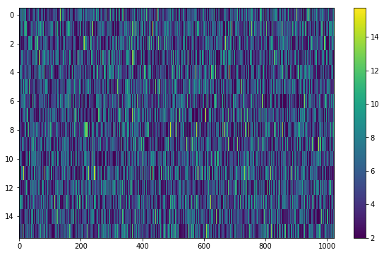
noise = frame.add_noise(x_mean=5, x_std=2, noise_type='gaussian')
fig = plt.figure(figsize=(10, 6))
plt.imshow(frame.get_data(), aspect='auto')
plt.colorbar()
plt.show()
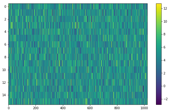
This adds Gaussian noise with mean 5 and standard deviation 2 to an empty frame.
In addition, we can truncate the noise at a lower bound specified by parameter x_min:
noise = frame.add_noise(x_mean=5, x_std=2, x_min=0, noise_type='gaussian')
This may be useful depending on the use case; you might not want negative intensities, or simply any intensity below a reasonable threshold, to occur in your synthetic data.
Adding synthetic noise based on real observations
We can also generate synthetic noise whose parameters are sampled from real observations. Specifically, we can select the mean for chi-squared noise, or additionally the standard deviation and minimum for Gaussian noise, from distributions of parameters estimated from observations.
If no distributions are provided by the user, noise parameters are sampled by
default from pre-loaded distributions in setigen. These were estimated
from GBT C-Band observations on frames with (dt, df) = (1.4 s, 1.4 Hz) and
(tchans, fchans) = (32, 1024). Behind the scenes, the mean, standard deviation,
and minimum intensity over each sub-frame in the observation were saved into
three respective numpy arrays.
The frame.add_noise_from_obs function also uses chi-squared noise by default,
selecting a mean intensity from the sampled observational distribution of means, and
populating the frame with chi-squared noise accordingly.
Alternately, by setting noise_type=gaussian or noise_type=normal
the function will select a mean, standard deviation, and minimum from these arrays (not
necessarily all corresponding to the same original observational sub-frame), and
populates your frame with Gaussian noise. You can also set the
share_index parameter to True, to force these random noise parameter selections
to all correspond to the same original observational sub-frame.
Note that these pre-loaded observations only serve as approximations and real observations vary depending on the noise temperature and frequency band. To be safe, you can generate your own parameters distributions from observational data.
For chi-squared noise:
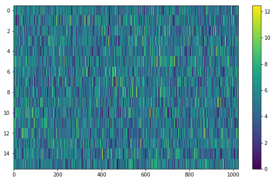
noise = frame.add_noise_from_obs()
We can readily see that the intensities are similar to a real GBT observation’s.
For Gaussian noise:
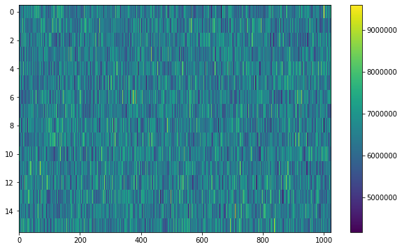
noise = frame.add_noise_from_obs(noise_type='gaussian')
We can also specify the distributions from which to sample parameters, one each for the mean, standard deviation, and minimum, as below. Note: just as in the pure noise generation above, you don’t need to specify an x_min_array from which to sample if there’s no need to truncate the noise at a lower bound.
noise = frame.add_noise_from_obs(x_mean_array=[3,4,5],
                                 x_std_array=[1,2,3],
                                 x_min_array=[1,2],
                                 share_index=False,
                                 noise_type='gaussian')
For chi-squared noise, only x_mean_array is used. For Gaussian noise, by default,
random noise parameter selections are forced to use the same indices (as opposed
to randomly choosing a parameter from each array) via share_index=True.
Convenience functions for signal generation
There are a few functions included in Frame that can help in constructing synthetic
signals.
Getting frame data
To just grab the underlying intensity data, you can do
data = frame.get_data(use_db=False)
As it implies, if you switch the use_db flag to true, it will express
the intensities in terms of decibels. This can help visualize data a little better,
depending on the application.
Plotting frames
Examples of the built-in plotting utilities are on the Getting started page:
frame.render()
frame.bl_render()
Note that both of these methods use matplotlib.pyplot.imshow behind
the scenes, which means you can still control plot parameters before and after
these function calls, e.g.
fig = plt.figure(figsize=(10, 6))
frame.render()
plt.title('My awesome title')
plt.savefig('frame.png')
plt.show()
SNR <-> Intensity
If a frame has background noise, we can calculate intensities corresponding to
different signal-to-noise (SNR) values. Here, the SNR of a signal is obtained
from integrating over the entire time axis, e.g. so that it reduces noise by
sqrt(tchans).
For example, the included signal parameter functions in setigen all calculate
signals based on absolute intensities, so if you’d like to include a signal with
an SNR of 10, you would do:
intensity = frame.get_intensity(snr=10)
Alternately, you can get the SNR of a given intensity by doing:
snr = frame.get_snr(intensity=100)
Frequency <-> Index
Another useful conversion is between frequencies and frame indices:
index = frame.get_index(frequency)
frequency = frame.get_frequency(index)
Drift rate
For some injection tasks, you might want to define signals based on where they
start and end on the frequency axis. Furthermore, this might not depend on
frequency per se. In these cases, you can calculate a drift frequency using the
get_drift_rate method:
start_index = np.random.randint(0, 1024)
end_index = np.random.randint(0, 1024)
drift_rate = frame.get_drift_rate(start_index, end_index)
Custom metadata
The Frame object includes a custom metadata property that allows you to manually
track injected signal parameters. Accordingly, frame.metadata is a simple
dictionary, making no assumptions about the type or number of signals you inject, or
even what information to store. This property is mainly included as an easy way to save the
data with the information you care about if you save and load frames with pickle.
new_metadata = {
    'snr': 10,
    'drift_rate': 2,
    'f_profile': 'lorentzian'
}

# Sets custom metadata to an input dictionary
frame.set_metadata(new_metadata)

# Appends input dictionary to custom metadata
frame.add_metadata(new_metadata)

# Gets custom metadata dict
metadata = frame.get_metadata()
Saving and loading frames
There are a few different ways to save information from frames.
Using pickle
Pickle lets us save and load entire Frame objects, which is helpful for keeping both data and metadata together in storage:
# Saving to file
frame.save_pickle(filename='frame.pickle')

# Loading a Frame object from file
loaded_frame = stg.Frame.load_pickle(filename='frame.pickle')
Note that load_pickle is a class method, not an instance method.
Using numpy
If you would only like to save the frame data as a numpy array, you can do:
frame.save_npy(filename='frame.npy')
This just uses the numpy.save and numpy.load functions to save
to .npy. If needed, you can also load in the data using
frame.load_npy(filename='frame.npy')
Using filterbank / HDF5
If you are interfacing with other Breakthrough Listen or astronomy codebases,
outputting setigen frames in filterbank or HDF5 format can be very useful. Note
that saving to HDF5 can have some difficulties based on your bitshuffle
installation and other dependencies, but saving as a filterbank file is stable.
We provide the following methods:
frame.save_fil(filename='frame.fil')
frame.save_hdf5(filename='frame.hdf5')
frame.save_h5(filename='frame.h5')
To get an equivalent blimpy Waterfall object in the same Python session,
use
waterfall = frame.get_waterfall()