Getting started

The heart of setigen is the Frame object. For signal injection and manipulation, we call each snippet of time-frequency data a “frame.” There are two main ways to initialize frames, starting from either resolution/size parameters or existing observational data.

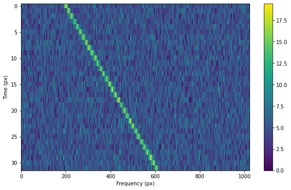
Here’s a minimal working example for a purely synthetic frame, injecting a constant intensity signal into a background of Gaussian noise. Parameters in setigen are specified either in terms of SI units (Hz, s) or astropy.units, as in the example:

from astropy import units as u
import setigen as stg
import matplotlib.pyplot as plt

frame = stg.Frame(fchans=1024*u.pixel,
                  tchans=32*u.pixel,
                  df=2.7939677238464355*u.Hz,
                  dt=18.25361108*u.s,
                  fch1=6095.214842353016*u.MHz)
frame.add_noise(x_mean=5, x_std=2, x_min=0)
frame.add_signal(stg.constant_path(f_start=frame.get_frequency(200),
                                   drift_rate=2*u.Hz/u.s),
                 stg.constant_t_profile(level=frame.get_intensity(snr=30)),
                 stg.gaussian_f_profile(width=40*u.Hz),
                 stg.constant_bp_profile(level=1))

fig = plt.figure(figsize=(10, 6))
frame.render()
plt.savefig('frame.png', bbox_inches='tight')
plt.show()

This simple signal can also be generated using the method frame.add_constant_signal, which is optimized for created signals of constant intensity and drift rate in large frames:

frame.add_constant_signal(f_start=frame.get_frequency(200),
                          drift_rate=2*u.Hz/u.s,
                          level=frame.get_intensity(snr=30),
                          width=40*u.Hz,
                          f_profile_type='gaussian')

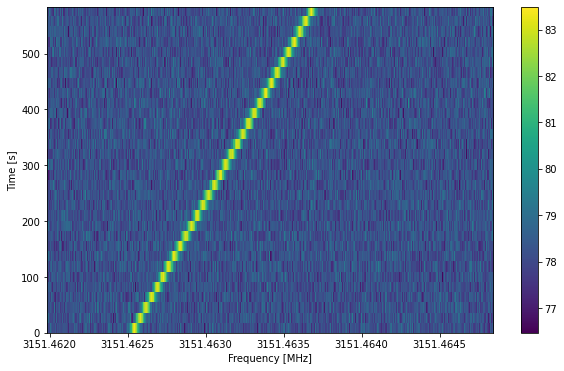
Similarly, here’s a minimal working example for injecting a signal into a frame of observational data (from a blimpy Waterfall object). Note that in this example, the observational data also has dimensions 32x1024 to make it easy to visualize here.

from astropy import units as u
import setigen as stg
import blimpy as bl
import matplotlib.pyplot as plt

data_path = 'path/to/data.fil'
waterfall = bl.Waterfall(data_path)
frame = stg.Frame(waterfall=waterfall)
frame.add_signal(stg.constant_path(f_start=frame.get_frequency(200),
                                   drift_rate=2*u.Hz/u.s),
                 stg.constant_t_profile(level=frame.get_intensity(snr=30)),
                 stg.gaussian_f_profile(width=40*u.Hz),
                 stg.constant_bp_profile(level=1))

fig = plt.figure(figsize=(10, 6))
frame.render()
plt.show()

We can also view this using blimpy’s plotting style:

fig = plt.figure(figsize=(10, 6))
frame.bl_render()
plt.show()